Creation of an InputsModel object for a airGRiwrm network
CreateInputsModel.GRiwrm.RdCreation of an InputsModel object for a airGRiwrm network
# S3 method for GRiwrm
CreateInputsModel(
  x,
  DatesR,
  Precip = NULL,
  PotEvap = NULL,
  Qobs = NULL,
  PrecipScale = TRUE,
  TempMean = NULL,
  TempMin = NULL,
  TempMax = NULL,
  ZInputs = NULL,
  HypsoData = NULL,
  NLayers = 5,
  ...
)
Arguments
- x
[GRiwrm object] diagram of the semi-distributed model (See CreateGRiwrm)
- DatesR
POSIXt vector of dates
- Precip
(optional) matrix or data.frame frame of numeric containing precipitation in [mm per time step]. Column names correspond to node IDs
- PotEvap
(optional) matrix or data.frame frame of numeric containing potential evaporation [mm per time step]. Column names correspond to node IDs
- Qobs
(optional) matrix or data.frame frame of numeric containing observed flows in [mm per time step]. Column names correspond to node IDs
- PrecipScale
(optional) named vector of logical indicating if the mean of the precipitation interpolated on the elevation layers must be kept or not, required to create CemaNeige module inputs, default
TRUE(the mean of the precipitation is kept to the original value)- TempMean
(optional) matrix or data.frame of time series of mean air temperature [°C], required to create the CemaNeige module inputs
- TempMin
(optional) matrix or data.frame of time series of minimum air temperature [°C], possibly used to create the CemaNeige module inputs
- TempMax
(optional) matrix or data.frame of time series of maximum air temperature [°C], possibly used to create the CemaNeige module inputs
- ZInputs
(optional) named vector of numeric giving the mean elevation of the Precip and Temp series (before extrapolation) [m], possibly used to create the CemaNeige module input
- HypsoData
(optional) matrix or data.frame containing 101 numeric rows: min, q01 to q99 and max of catchment elevation distribution [m], if not defined a single elevation is used for CemaNeige
- NLayers
(optional) named vector of numeric integer giving the number of elevation layers requested -, required to create CemaNeige module inputs, default=5
- ...
used for compatibility with S3 methods
Value
A GRiwrmInputsModel object which is a list of InputsModel objects created by airGR::CreateInputsModel with one item per modeled sub-catchment.
Details
Meteorological data are needed for the nodes of the network that represent a catchment simulated by a rainfall-runoff model. Instead of airGR::CreateInputsModel that has numeric vector as time series inputs, this function uses matrix or data.frame with the id of the sub-catchment as column names. For single values (ZInputs or NLayers), the function requires named vector with the id of the sub-catchment as name item. If an argument is optional, only the column or the named item has to be provided.
See airGR::CreateInputsModel documentation for details concerning each input.
Examples
###################################################################
# Run the `airGR::RunModel_Lag` example in the GRiwrm fashion way #
# Simulation of a reservoir with a purpose of low-flow mitigation #
###################################################################
## ---- preparation of the InputsModel object
## loading package and catchment data
library(airGRiwrm)
data(L0123001)
## ---- specifications of the reservoir
## the reservoir withdraws 1 m3/s when it's possible considering the flow observed in the basin
Qupstream <- matrix(-sapply(BasinObs$Qls / 1000 - 1, function(x) {
min(1, max(0, x, na.rm = TRUE))
}), ncol = 1)
## except between July and September when the reservoir releases 3 m3/s for low-flow mitigation
month <- as.numeric(format(BasinObs$DatesR, "%m"))
Qupstream[month >= 7 & month <= 9] <- 3
Qupstream <- Qupstream * 86400 ## Conversion in m3/day
## the reservoir is not an upstream subcachment: its areas is NA
BasinAreas <- c(NA, BasinInfo$BasinArea)
## delay time between the reservoir and the catchment outlet is 2 days and the distance is 150 km
LengthHydro <- 150
## with a delay of 2 days for 150 km, the flow velocity is 75 km per day
Velocity <- (LengthHydro * 1e3 / 2) / (24 * 60 * 60) ## Conversion km/day -> m/s
# This example is a network of 2 nodes which can be describe like this:
db <- data.frame(id = c("Reservoir", "GaugingDown"),
length = c(LengthHydro, NA),
down = c("GaugingDown", NA),
area = c(NA, BasinInfo$BasinArea),
model = c(NA, "RunModel_GR4J"),
stringsAsFactors = FALSE)
# Create GRiwrm object from the data.frame
griwrm <- CreateGRiwrm(db)
str(griwrm)
#> Classes 'GRiwrm' and 'data.frame': 2 obs. of 5 variables:
#> $ id : chr "Reservoir" "GaugingDown"
#> $ down : chr "GaugingDown" NA
#> $ length: num 150 NA
#> $ model : chr NA "RunModel_GR4J"
#> $ area : num NA 360
# Formatting observations for the hydrological models
# Each input data should be a matrix or a data.frame with the good id in the name of the column
Precip <- matrix(BasinObs$P, ncol = 1)
colnames(Precip) <- "GaugingDown"
PotEvap <- matrix(BasinObs$E, ncol = 1)
colnames(PotEvap) <- "GaugingDown"
# Observed flows contain flows that are directly injected in the model
Qobs = matrix(Qupstream, ncol = 1)
colnames(Qobs) <- "Reservoir"
# Creation of the GRiwrmInputsModel object (= a named list of InputsModel objects)
InputsModels <- CreateInputsModel(griwrm,
DatesR = BasinObs$DatesR,
Precip = Precip,
PotEvap = PotEvap,
Qobs = Qobs)
#> CreateInputsModel.GRiwrm: Treating sub-basin GaugingDown...
str(InputsModels)
#> List of 1
#> $ GaugingDown:List of 11
#> ..$ DatesR : POSIXlt[1:10593], format: "1984-01-01" "1984-01-02" ...
#> ..$ Precip : num [1:10593] 4.1 15.9 0.8 0 0 0 0 0 2.9 0 ...
#> ..$ PotEvap : num [1:10593] 0.2 0.2 0.3 0.3 0.1 0.3 0.4 0.4 0.5 0.5 ...
#> ..$ Qupstream : num [1:10593, 1] -86400 -86400 -86400 -86400 -86400 -86400 -86400 -86400 -86400 -86400 ...
#> .. ..- attr(*, "dimnames")=List of 2
#> .. .. ..$ : NULL
#> .. .. ..$ : chr "Reservoir"
#> ..$ LengthHydro : Named num 150
#> .. ..- attr(*, "names")= chr "Reservoir"
#> ..$ BasinAreas : Named num [1:2] NA 360
#> .. ..- attr(*, "names")= chr [1:2] "Reservoir" "GaugingDown"
#> ..$ id : chr "GaugingDown"
#> ..$ down : chr NA
#> ..$ UpstreamNodes : chr "Reservoir"
#> ..$ UpstreamIsRunoff: logi FALSE
#> ..$ FUN_MOD : chr "RunModel_GR4J"
#> ..- attr(*, "class")= chr [1:4] "InputsModel" "daily" "GR" "SD"
#> - attr(*, "class")= chr [1:2] "GRiwrmInputsModel" "list"
#> - attr(*, "GRiwrm")=Classes 'GRiwrm' and 'data.frame': 2 obs. of 5 variables:
#> ..$ id : chr [1:2] "Reservoir" "GaugingDown"
#> ..$ down : chr [1:2] "GaugingDown" NA
#> ..$ length: num [1:2] 150 NA
#> ..$ model : chr [1:2] NA "RunModel_GR4J"
#> ..$ area : num [1:2] NA 360
#> - attr(*, "TimeStep")= num 86400
## run period selection
Ind_Run <- seq(which(format(BasinObs$DatesR, format = "%Y-%m-%d")=="1990-01-01"),
which(format(BasinObs$DatesR, format = "%Y-%m-%d")=="1999-12-31"))
# Creation of the GriwmRunOptions object
RunOptions <- CreateRunOptions(InputsModels,
IndPeriod_Run = Ind_Run)
#> Warning: model warm up period not defined: default configuration used
#> the year preceding the run period is used
str(RunOptions)
#> List of 1
#> $ GaugingDown:List of 8
#> ..$ IndPeriod_WarmUp: int [1:365] 1828 1829 1830 1831 1832 1833 1834 1835 1836 1837 ...
#> ..$ IndPeriod_Run : int [1:3652] 2193 2194 2195 2196 2197 2198 2199 2200 2201 2202 ...
#> ..$ IniStates : num [1:67] 0 0 0 0 0 0 0 0 0 0 ...
#> ..$ IniResLevels : num [1:4] 0.3 0.5 NA NA
#> ..$ Outputs_Cal : chr [1:2] "Qsim" "Param"
#> ..$ Outputs_Sim : Named chr [1:24] "DatesR" "PotEvap" "Precip" "Prod" ...
#> .. ..- attr(*, "names")= chr [1:24] "" "GR1" "GR2" "GR3" ...
#> ..$ FortranOutputs :List of 2
#> .. ..$ GR: chr [1:18] "PotEvap" "Precip" "Prod" "Pn" ...
#> .. ..$ CN: NULL
#> ..$ FeatFUN_MOD :List of 12
#> .. ..$ CodeMod : chr "GR4J"
#> .. ..$ NameMod : chr "GR4J"
#> .. ..$ NbParam : num 5
#> .. ..$ TimeUnit : chr "daily"
#> .. ..$ Id : logi NA
#> .. ..$ Class : chr [1:2] "daily" "GR"
#> .. ..$ Pkg : chr "airGR"
#> .. ..$ NameFunMod : chr "RunModel_GR4J"
#> .. ..$ TimeStep : num 86400
#> .. ..$ TimeStepMean: int 86400
#> .. ..$ CodeModHydro: chr "GR4J"
#> .. ..$ IsSD : logi TRUE
#> ..- attr(*, "class")= chr [1:3] "RunOptions" "daily" "GR"
#> - attr(*, "class")= chr [1:2] "list" "GRiwrmRunOptions"
# Parameters of the SD models should be encapsulated in a named list
ParamGR4J <- c(X1 = 257.238, X2 = 1.012, X3 = 88.235, X4 = 2.208)
Param <- list(`GaugingDown` = c(Velocity, ParamGR4J))
# RunModel for the whole network
OutputsModels <- RunModel(InputsModels,
RunOptions = RunOptions,
Param = Param)
#> RunModel.GRiwrmInputsModel: Treating sub-basin GaugingDown...
str(OutputsModels)
#> List of 1
#> $ GaugingDown:List of 23
#> ..$ DatesR : POSIXlt[1:3652], format: "1990-01-01" "1990-01-02" ...
#> ..$ PotEvap : num [1:3652] 0.3 0.4 0.4 0.3 0.1 0.1 0.1 0.2 0.2 0.3 ...
#> ..$ Precip : num [1:3652] 0 9.3 3.2 7.3 0 0 0 0 0.1 0.2 ...
#> ..$ Prod : num [1:3652] 196 199 199 201 200 ...
#> ..$ Pn : num [1:3652] 0 8.9 2.8 7 0 0 0 0 0 0 ...
#> ..$ Ps : num [1:3652] 0 3.65 1.12 2.75 0 ...
#> ..$ AE : num [1:3652] 0.2833 0.4 0.4 0.3 0.0952 ...
#> ..$ Perc : num [1:3652] 0.645 0.696 0.703 0.74 0.725 ...
#> ..$ PR : num [1:3652] 0.645 5.946 2.383 4.992 0.725 ...
#> ..$ Q9 : num [1:3652] 1.78 1.52 3.86 3.17 3.45 ...
#> ..$ Q1 : num [1:3652] 0.2 0.195 0.271 0.387 0.365 ...
#> ..$ Rout : num [1:3652] 53.9 53.6 55.3 56.1 56.9 ...
#> ..$ Exch : num [1:3652] 0.181 0.18 0.176 0.197 0.207 ...
#> ..$ AExch1 : num [1:3652] 0.181 0.18 0.176 0.197 0.207 ...
#> ..$ AExch2 : num [1:3652] 0.181 0.18 0.176 0.197 0.207 ...
#> ..$ AExch : num [1:3652] 0.362 0.36 0.353 0.393 0.414 ...
#> ..$ QR : num [1:3652] 2.05 1.99 2.36 2.55 2.78 ...
#> ..$ QD : num [1:3652] 0.381 0.375 0.447 0.584 0.572 ...
#> ..$ Qsim : num [1:3652] 2.43 2.37 2.56 2.9 3.11 ...
#> ..$ RunOptions:List of 3
#> .. ..$ WarmUpQsim : num [1:365] 0.539 0.575 0.807 0.731 0.674 ...
#> .. ..$ Param : Named num [1:5] 0.868 257.238 1.012 88.235 2.208
#> .. .. ..- attr(*, "names")= chr [1:5] "" "" "" "" ...
#> .. ..$ WarmUpQsim_m3: num [1:365] NA NA NA NA NA NA NA NA NA NA ...
#> ..$ StateEnd :List of 4
#> .. ..$ Store :List of 4
#> .. .. ..$ Prod: num 189
#> .. .. ..$ Rout: num 48.9
#> .. .. ..$ Exp : num NA
#> .. .. ..$ Int : num NA
#> .. ..$ UH :List of 2
#> .. .. ..$ UH1: num [1:20] 0.514 0.54 0.148 0 0 ...
#> .. .. ..$ UH2: num [1:40] 0.056306 0.057176 0.042254 0.012188 0.000578 ...
#> .. ..$ CemaNeigeLayers:List of 4
#> .. .. ..$ G : num NA
#> .. .. ..$ eTG : num NA
#> .. .. ..$ Gthr : num NA
#> .. .. ..$ Glocmax: num NA
#> .. ..$ SD :List of 1
#> .. .. ..$ : num [1:3] -86400 -86400 -86400
#> .. ..- attr(*, "class")= chr [1:3] "IniStates" "daily" "GR"
#> ..$ Qsim_m3 : num [1:3652] 875333 851839 922461 1042434 1119947 ...
#> ..$ QsimDown : num [1:3652] 2.43 2.37 2.8 3.14 3.35 ...
#> ..- attr(*, "class")= chr [1:4] "OutputsModel" "daily" "GR" "SD"
#> - attr(*, "class")= chr [1:2] "GRiwrmOutputsModel" "list"
#> - attr(*, "Qm3s")=Classes 'Qm3s' and 'data.frame': 3652 obs. of 3 variables:
#> ..$ DatesR : POSIXct[1:3652], format: "1990-01-01" "1990-01-02" ...
#> ..$ Reservoir : num [1:3652] -1 -1 -1 -1 -1 -1 -1 -1 -1 -1 ...
#> ..$ GaugingDown: num [1:3652] 10.13 9.86 10.68 12.07 12.96 ...
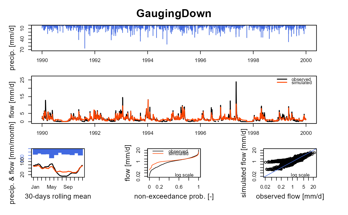
# Compare Simulation with reservoir and observation of natural flow
plot(OutputsModels, data.frame(GaugingDown = BasinObs$Qmm[Ind_Run]))