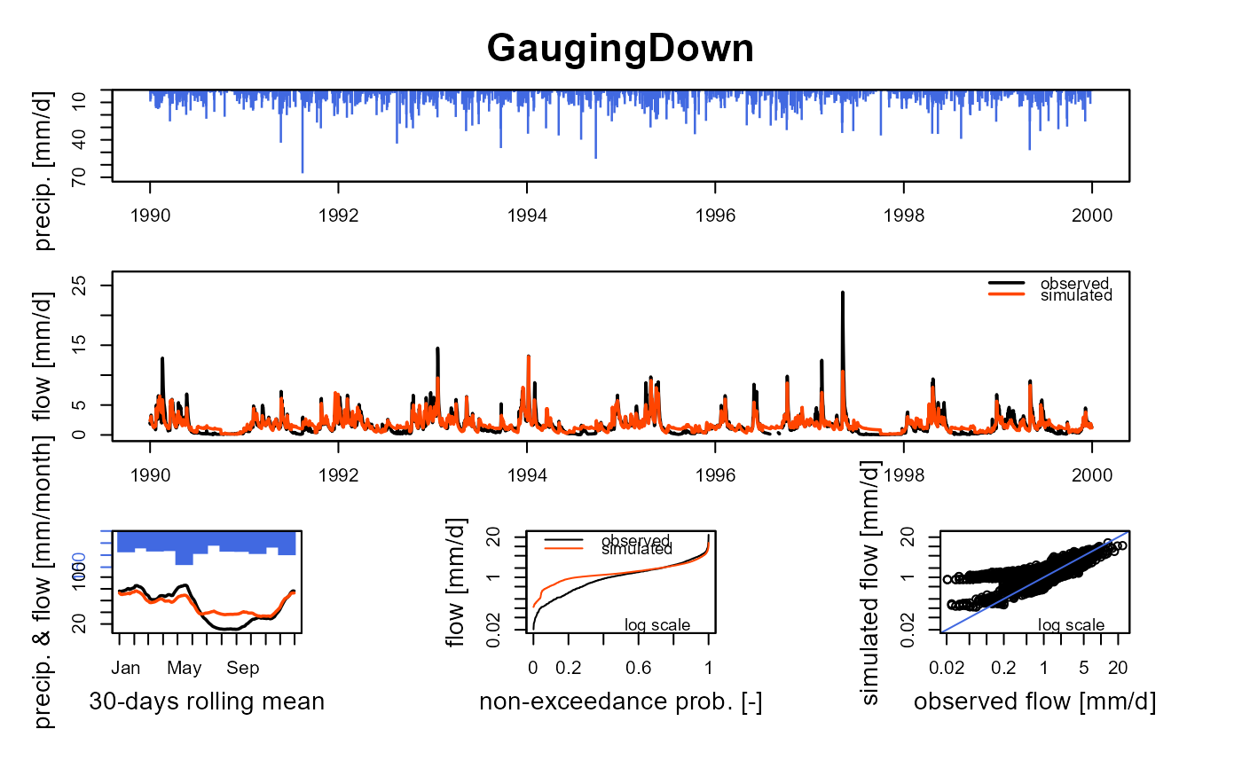
Function which creates screen plots giving an overview of the model outputs in the GRiwrm network
plot.GRiwrmOutputsModel.RdFunction which creates screen plots giving an overview of the model outputs in the GRiwrm network
# S3 method for GRiwrmOutputsModel
plot(x, Qobs = NULL, ...)
Arguments
- x
[object of class GRiwrmOutputsModel] see RunModel.GRiwrmInputsModel for details
- Qobs
(optional) matrix time series of observed flows (for the same time steps than simulated) (mm/time step) with one column by hydrological model output named with the node ID (See CreateGRiwrm for details)
- ...
Further arguments for airGR::plot.OutputsModel and plot
Value
list of plots.
Examples
###################################################################
# Run the `airGR::RunModel_Lag` example in the GRiwrm fashion way #
# Simulation of a reservoir with a purpose of low-flow mitigation #
###################################################################

## ---- preparation of the InputsModel object

## loading package and catchment data
library(airGRiwrm)
data(L0123001)

## ---- specifications of the reservoir

## the reservoir withdraws 1 m3/s when it's possible considering the flow observed in the basin
Qupstream <- matrix(-sapply(BasinObs$Qls / 1000 - 1, function(x) {
  min(1, max(0, x, na.rm = TRUE))
}), ncol = 1)

## except between July and September when the reservoir releases 3 m3/s for low-flow mitigation
month <- as.numeric(format(BasinObs$DatesR, "%m"))
Qupstream[month >= 7 & month <= 9] <- 3
Qupstream <- Qupstream * 86400 ## Conversion in m3/day

## the reservoir is not an upstream subcachment: its areas is NA
BasinAreas <- c(NA, BasinInfo$BasinArea)

## delay time between the reservoir and the catchment outlet is 2 days and the distance is 150 km
LengthHydro <- 150
## with a delay of 2 days for 150 km, the flow velocity is 75 km per day
Velocity <- (LengthHydro * 1e3 / 2) / (24 * 60 * 60) ## Conversion km/day -> m/s

# This example is a network of 2 nodes which can be describe like this:
db <- data.frame(id = c("Reservoir", "GaugingDown"),
                 length = c(LengthHydro, NA),
                 down = c("GaugingDown", NA),
                 area = c(NA, BasinInfo$BasinArea),
                 model = c(NA, "RunModel_GR4J"),
                 stringsAsFactors = FALSE)

# Create GRiwrm object from the data.frame
griwrm <- CreateGRiwrm(db)
str(griwrm)
#> Classes 'GRiwrm' and 'data.frame':	2 obs. of  5 variables:
#>  $ id    : chr  "Reservoir" "GaugingDown"
#>  $ down  : chr  "GaugingDown" NA
#>  $ length: num  150 NA
#>  $ model : chr  NA "RunModel_GR4J"
#>  $ area  : num  NA 360

# Formatting observations for the hydrological models
# Each input data should be a matrix or a data.frame with the good id in the name of the column
Precip <- matrix(BasinObs$P, ncol = 1)
colnames(Precip) <- "GaugingDown"
PotEvap <- matrix(BasinObs$E, ncol = 1)
colnames(PotEvap) <- "GaugingDown"

# Observed flows contain flows that are directly injected in the model
Qobs = matrix(Qupstream, ncol = 1)
colnames(Qobs) <- "Reservoir"

# Creation of the GRiwrmInputsModel object (= a named list of InputsModel objects)
InputsModels <- CreateInputsModel(griwrm,
                            DatesR = BasinObs$DatesR,
                            Precip = Precip,
                            PotEvap = PotEvap,
                            Qobs = Qobs)
#> CreateInputsModel.GRiwrm: Treating sub-basin GaugingDown...
str(InputsModels)
#> List of 1
#>  $ GaugingDown:List of 11
#>   ..$ DatesR          : POSIXlt[1:10593], format: "1984-01-01" "1984-01-02" ...
#>   ..$ Precip          : num [1:10593] 4.1 15.9 0.8 0 0 0 0 0 2.9 0 ...
#>   ..$ PotEvap         : num [1:10593] 0.2 0.2 0.3 0.3 0.1 0.3 0.4 0.4 0.5 0.5 ...
#>   ..$ Qupstream       : num [1:10593, 1] -86400 -86400 -86400 -86400 -86400 -86400 -86400 -86400 -86400 -86400 ...
#>   .. ..- attr(*, "dimnames")=List of 2
#>   .. .. ..$ : NULL
#>   .. .. ..$ : chr "Reservoir"
#>   ..$ LengthHydro     : Named num 150
#>   .. ..- attr(*, "names")= chr "Reservoir"
#>   ..$ BasinAreas      : Named num [1:2] NA 360
#>   .. ..- attr(*, "names")= chr [1:2] "Reservoir" "GaugingDown"
#>   ..$ id              : chr "GaugingDown"
#>   ..$ down            : chr NA
#>   ..$ UpstreamNodes   : chr "Reservoir"
#>   ..$ UpstreamIsRunoff: logi FALSE
#>   ..$ FUN_MOD         : chr "RunModel_GR4J"
#>   ..- attr(*, "class")= chr [1:4] "InputsModel" "daily" "GR" "SD"
#>  - attr(*, "class")= chr [1:2] "GRiwrmInputsModel" "list"
#>  - attr(*, "GRiwrm")=Classes 'GRiwrm' and 'data.frame':	2 obs. of  5 variables:
#>   ..$ id    : chr [1:2] "Reservoir" "GaugingDown"
#>   ..$ down  : chr [1:2] "GaugingDown" NA
#>   ..$ length: num [1:2] 150 NA
#>   ..$ model : chr [1:2] NA "RunModel_GR4J"
#>   ..$ area  : num [1:2] NA 360
#>  - attr(*, "TimeStep")= num 86400

## run period selection
Ind_Run <- seq(which(format(BasinObs$DatesR, format = "%Y-%m-%d")=="1990-01-01"),
               which(format(BasinObs$DatesR, format = "%Y-%m-%d")=="1999-12-31"))

# Creation of the GriwmRunOptions object
RunOptions <- CreateRunOptions(InputsModels,
                                IndPeriod_Run = Ind_Run)
#> Warning: model warm up period not defined: default configuration used
#>   the year preceding the run period is used
str(RunOptions)
#> List of 1
#>  $ GaugingDown:List of 8
#>   ..$ IndPeriod_WarmUp: int [1:365] 1828 1829 1830 1831 1832 1833 1834 1835 1836 1837 ...
#>   ..$ IndPeriod_Run   : int [1:3652] 2193 2194 2195 2196 2197 2198 2199 2200 2201 2202 ...
#>   ..$ IniStates       : num [1:67] 0 0 0 0 0 0 0 0 0 0 ...
#>   ..$ IniResLevels    : num [1:4] 0.3 0.5 NA NA
#>   ..$ Outputs_Cal     : chr [1:2] "Qsim" "Param"
#>   ..$ Outputs_Sim     : Named chr [1:24] "DatesR" "PotEvap" "Precip" "Prod" ...
#>   .. ..- attr(*, "names")= chr [1:24] "" "GR1" "GR2" "GR3" ...
#>   ..$ FortranOutputs  :List of 2
#>   .. ..$ GR: chr [1:18] "PotEvap" "Precip" "Prod" "Pn" ...
#>   .. ..$ CN: NULL
#>   ..$ FeatFUN_MOD     :List of 12
#>   .. ..$ CodeMod     : chr "GR4J"
#>   .. ..$ NameMod     : chr "GR4J"
#>   .. ..$ NbParam     : num 5
#>   .. ..$ TimeUnit    : chr "daily"
#>   .. ..$ Id          : logi NA
#>   .. ..$ Class       : chr [1:2] "daily" "GR"
#>   .. ..$ Pkg         : chr "airGR"
#>   .. ..$ NameFunMod  : chr "RunModel_GR4J"
#>   .. ..$ TimeStep    : num 86400
#>   .. ..$ TimeStepMean: int 86400
#>   .. ..$ CodeModHydro: chr "GR4J"
#>   .. ..$ IsSD        : logi TRUE
#>   ..- attr(*, "class")= chr [1:3] "RunOptions" "daily" "GR"
#>  - attr(*, "class")= chr [1:2] "list" "GRiwrmRunOptions"

# Parameters of the SD models should be encapsulated in a named list
ParamGR4J <- c(X1 = 257.238, X2 = 1.012, X3 = 88.235, X4 = 2.208)
Param <- list(`GaugingDown` = c(Velocity, ParamGR4J))

# RunModel for the whole network
OutputsModels <- RunModel(InputsModels,
                          RunOptions = RunOptions,
                          Param = Param)
#> RunModel.GRiwrmInputsModel: Treating sub-basin GaugingDown...
str(OutputsModels)
#> List of 1
#>  $ GaugingDown:List of 23
#>   ..$ DatesR    : POSIXlt[1:3652], format: "1990-01-01" "1990-01-02" ...
#>   ..$ PotEvap   : num [1:3652] 0.3 0.4 0.4 0.3 0.1 0.1 0.1 0.2 0.2 0.3 ...
#>   ..$ Precip    : num [1:3652] 0 9.3 3.2 7.3 0 0 0 0 0.1 0.2 ...
#>   ..$ Prod      : num [1:3652] 196 199 199 201 200 ...
#>   ..$ Pn        : num [1:3652] 0 8.9 2.8 7 0 0 0 0 0 0 ...
#>   ..$ Ps        : num [1:3652] 0 3.65 1.12 2.75 0 ...
#>   ..$ AE        : num [1:3652] 0.2833 0.4 0.4 0.3 0.0952 ...
#>   ..$ Perc      : num [1:3652] 0.645 0.696 0.703 0.74 0.725 ...
#>   ..$ PR        : num [1:3652] 0.645 5.946 2.383 4.992 0.725 ...
#>   ..$ Q9        : num [1:3652] 1.78 1.52 3.86 3.17 3.45 ...
#>   ..$ Q1        : num [1:3652] 0.2 0.195 0.271 0.387 0.365 ...
#>   ..$ Rout      : num [1:3652] 53.9 53.6 55.3 56.1 56.9 ...
#>   ..$ Exch      : num [1:3652] 0.181 0.18 0.176 0.197 0.207 ...
#>   ..$ AExch1    : num [1:3652] 0.181 0.18 0.176 0.197 0.207 ...
#>   ..$ AExch2    : num [1:3652] 0.181 0.18 0.176 0.197 0.207 ...
#>   ..$ AExch     : num [1:3652] 0.362 0.36 0.353 0.393 0.414 ...
#>   ..$ QR        : num [1:3652] 2.05 1.99 2.36 2.55 2.78 ...
#>   ..$ QD        : num [1:3652] 0.381 0.375 0.447 0.584 0.572 ...
#>   ..$ Qsim      : num [1:3652] 2.43 2.37 2.56 2.9 3.11 ...
#>   ..$ RunOptions:List of 3
#>   .. ..$ WarmUpQsim   : num [1:365] 0.539 0.575 0.807 0.731 0.674 ...
#>   .. ..$ Param        : Named num [1:5] 0.868 257.238 1.012 88.235 2.208
#>   .. .. ..- attr(*, "names")= chr [1:5] "" "" "" "" ...
#>   .. ..$ WarmUpQsim_m3: num [1:365] NA NA NA NA NA NA NA NA NA NA ...
#>   ..$ StateEnd  :List of 4
#>   .. ..$ Store          :List of 4
#>   .. .. ..$ Prod: num 189
#>   .. .. ..$ Rout: num 48.9
#>   .. .. ..$ Exp : num NA
#>   .. .. ..$ Int : num NA
#>   .. ..$ UH             :List of 2
#>   .. .. ..$ UH1: num [1:20] 0.514 0.54 0.148 0 0 ...
#>   .. .. ..$ UH2: num [1:40] 0.056306 0.057176 0.042254 0.012188 0.000578 ...
#>   .. ..$ CemaNeigeLayers:List of 4
#>   .. .. ..$ G      : num NA
#>   .. .. ..$ eTG    : num NA
#>   .. .. ..$ Gthr   : num NA
#>   .. .. ..$ Glocmax: num NA
#>   .. ..$ SD             :List of 1
#>   .. .. ..$ : num [1:3] -86400 -86400 -86400
#>   .. ..- attr(*, "class")= chr [1:3] "IniStates" "daily" "GR"
#>   ..$ Qsim_m3   : num [1:3652] 875333 851839 922461 1042434 1119947 ...
#>   ..$ QsimDown  : num [1:3652] 2.43 2.37 2.8 3.14 3.35 ...
#>   ..- attr(*, "class")= chr [1:4] "OutputsModel" "daily" "GR" "SD"
#>  - attr(*, "class")= chr [1:2] "GRiwrmOutputsModel" "list"
#>  - attr(*, "Qm3s")=Classes 'Qm3s' and 'data.frame':	3652 obs. of  3 variables:
#>   ..$ DatesR     : POSIXct[1:3652], format: "1990-01-01" "1990-01-02" ...
#>   ..$ Reservoir  : num [1:3652] -1 -1 -1 -1 -1 -1 -1 -1 -1 -1 ...
#>   ..$ GaugingDown: num [1:3652] 10.13 9.86 10.68 12.07 12.96 ...

# Compare Simulation with reservoir and observation of natural flow
plot(OutputsModels, data.frame(GaugingDown = BasinObs$Qmm[Ind_Run]))