Creation of an InputsModel object for a airGRiwrm network
Source:R/CreateInputsModel.GRiwrm.R
CreateInputsModel.GRiwrm.RdCreation of an InputsModel object for a airGRiwrm network
# S3 method for GRiwrm
CreateInputsModel(
  x,
  DatesR,
  Precip = NULL,
  PotEvap = NULL,
  Qobs = NULL,
  Qmin = NULL,
  PrecipScale = TRUE,
  TempMean = NULL,
  TempMin = NULL,
  TempMax = NULL,
  ZInputs = NULL,
  HypsoData = NULL,
  NLayers = 5,
  IsHyst = FALSE,
  ...
)
Arguments
- x
[GRiwrm object] diagram of the semi-distributed model (See CreateGRiwrm)
- DatesR
POSIXt vector of dates
- Precip
(optional) matrix or data.frame of numeric containing precipitation in [mm per time step]. Column names correspond to node IDs
- PotEvap
(optional) matrix or data.frame of numeric containing potential evaporation [mm per time step]. Column names correspond to node IDs
- Qobs
(optional) matrix or data.frame of numeric containing observed flows. It must be provided only for nodes of type "Direct injection" and "Diversion". See CreateGRiwrm for details about these node types. Unit is [mm per time step] for nodes with an area, and [m3 per time step] for nodes with
area=NA. Column names correspond to node IDs. Negative flows are abstracted from the model and positive flows are injected to the model- Qmin
(optional) matrix or data.frame of numeric containing minimum flows to let downstream of a node with a Diversion [m3 per time step]. Default is zero. Column names correspond to node IDs
- PrecipScale
(optional) named vector of logical indicating if the mean of the precipitation interpolated on the elevation layers must be kept or not, required to create CemaNeige module inputs, default
TRUE(the mean of the precipitation is kept to the original value)- TempMean
(optional) matrix or data.frame of time series of mean air temperature [°C], required to create the CemaNeige module inputs
- TempMin
(optional) matrix or data.frame of time series of minimum air temperature [°C], possibly used to create the CemaNeige module inputs
- TempMax
(optional) matrix or data.frame of time series of maximum air temperature [°C], possibly used to create the CemaNeige module inputs
- ZInputs
(optional) named vector of numeric giving the mean elevation of the Precip and Temp series (before extrapolation) [m], possibly used to create the CemaNeige module input
- HypsoData
(optional) matrix or data.frame containing 101 numeric rows: min, q01 to q99 and max of catchment elevation distribution [m], if not defined a single elevation is used for CemaNeige
- NLayers
(optional) named vector of numeric integer giving the number of elevation layers requested -, required to create CemaNeige module inputs, default=5
- IsHyst
logical boolean indicating if the hysteresis version of CemaNeige is used. See details of airGR::CreateRunOptions.
- ...
used for compatibility with S3 methods
Value
A GRiwrmInputsModel object which is a list of InputsModel
objects created by airGR::CreateInputsModel with one item per modeled sub-catchment.
Details
Meteorological data are needed for the nodes of the network that
represent a catchment simulated by a rainfall-runoff model. Instead of
airGR::CreateInputsModel that has numeric vector as time series inputs,
this function uses matrix or data.frame with the id of the sub-catchment
as column names. For single values (ZInputs or NLayers), the function
requires named vector with the id of the sub-catchment as name item. If an
argument is optional, only the column or the named item has to be provided.
See airGR::CreateInputsModel documentation for details concerning each input.
Number of rows of Precip, PotEvap, Qobs, Qmin, TempMean, TempMin,
TempMax must be the same of the length of DatesR (each row corresponds to
a time step defined in DatesR).
For example of use of Direct Injection nodes, see vignettes "V03_Open-loop_influenced_flow" and "V04_Closed-loop_regulated_withdrawal".
For example of use of Diversion nodes, see example below and vignette "V06_Modelling_regulated_diversion".
Examples
###################################################################
# Run the `airGR::RunModel_Lag` example in the GRiwrm fashion way #
# Simulation of a reservoir with a purpose of low-flow mitigation #
###################################################################
## ---- preparation of the InputsModel object
## loading package and catchment data
library(airGRiwrm)
data(L0123001)
## ---- specifications of the reservoir
## the reservoir withdraws 1 m3/s when it's possible considering the flow observed in the basin
Qupstream <- matrix(-sapply(BasinObs$Qls / 1000 - 1, function(x) {
min(1, max(0, x, na.rm = TRUE))
}), ncol = 1)
## except between July and September when the reservoir releases 3 m3/s for low-flow mitigation
month <- as.numeric(format(BasinObs$DatesR, "%m"))
Qupstream[month >= 7 & month <= 9] <- 3
Qupstream <- Qupstream * 86400 ## Conversion in m3/day
## the reservoir is not an upstream subcachment: its areas is NA
BasinAreas <- c(NA, BasinInfo$BasinArea)
## delay time between the reservoir and the catchment outlet is 2 days and the distance is 150 km
LengthHydro <- 150
## with a delay of 2 days for 150 km, the flow velocity is 75 km per day
Velocity <- (LengthHydro * 1e3 / 2) / (24 * 60 * 60) ## Conversion km/day -> m/s
# This example is a network of 2 nodes which can be describe like this:
db <- data.frame(id = c("Reservoir", "GaugingDown"),
length = c(LengthHydro, NA),
down = c("GaugingDown", NA),
area = c(NA, BasinInfo$BasinArea),
model = c(NA, "RunModel_GR4J"),
stringsAsFactors = FALSE)
# Create GRiwrm object from the data.frame
griwrm <- CreateGRiwrm(db)
plot(griwrm)
# Formatting observations for the hydrological models
# Each input data should be a matrix or a data.frame with the good id in the name of the column
Precip <- matrix(BasinObs$P, ncol = 1)
colnames(Precip) <- "GaugingDown"
PotEvap <- matrix(BasinObs$E, ncol = 1)
colnames(PotEvap) <- "GaugingDown"
# Observed flows contain flows that are directly injected in the model
Qobs = matrix(Qupstream, ncol = 1)
colnames(Qobs) <- "Reservoir"
# Creation of the GRiwrmInputsModel object (= a named list of InputsModel objects)
InputsModels <- CreateInputsModel(griwrm,
DatesR = BasinObs$DatesR,
Precip = Precip,
PotEvap = PotEvap,
Qobs = Qobs)
#> CreateInputsModel.GRiwrm: Processing sub-basin GaugingDown...
str(InputsModels)
#> List of 1
#> $ GaugingDown:List of 18
#> ..$ DatesR : POSIXlt[1:10593], format: "1984-01-01" "1984-01-02" ...
#> ..$ Precip : num [1:10593] 4.1 15.9 0.8 0 0 0 0 0 2.9 0 ...
#> ..$ PotEvap : num [1:10593] 0.2 0.2 0.3 0.3 0.1 0.3 0.4 0.4 0.5 0.5 ...
#> ..$ Qupstream : num [1:10593, 1] -86400 -86400 -86400 -86400 -86400 -86400 -86400 -86400 -86400 -86400 ...
#> .. ..- attr(*, "dimnames")=List of 2
#> .. .. ..$ : NULL
#> .. .. ..$ : chr "Reservoir"
#> ..$ LengthHydro : Named num 150
#> .. ..- attr(*, "names")= chr "Reservoir"
#> ..$ BasinAreas : Named num [1:2] NA 360
#> .. ..- attr(*, "names")= chr [1:2] "Reservoir" "GaugingDown"
#> ..$ id : chr "GaugingDown"
#> ..$ down : chr NA
#> ..$ UpstreamNodes : chr "Reservoir"
#> ..$ UpstreamIsModeled: Named logi FALSE
#> .. ..- attr(*, "names")= chr "Reservoir"
#> ..$ UpstreamVarQ : Named chr "Qsim_m3"
#> .. ..- attr(*, "names")= chr "Reservoir"
#> ..$ FUN_MOD : chr "RunModel_GR4J"
#> ..$ isUngauged : logi FALSE
#> ..$ gaugedId : chr "GaugingDown"
#> ..$ hasUngaugedNodes : logi FALSE
#> ..$ model :List of 4
#> .. ..$ indexParamUngauged: num [1:5] 1 2 3 4 5
#> .. ..$ hasX4 : logi TRUE
#> .. ..$ iX4 : num 5
#> .. ..$ IsHyst : logi FALSE
#> ..$ hasDiversion : logi FALSE
#> ..$ isReservoir : logi FALSE
#> ..- attr(*, "class")= chr [1:4] "InputsModel" "daily" "GR" "SD"
#> - attr(*, "class")= chr [1:2] "GRiwrmInputsModel" "list"
#> - attr(*, "GRiwrm")=Classes ‘GRiwrm’ and 'data.frame': 2 obs. of 6 variables:
#> ..$ id : chr [1:2] "Reservoir" "GaugingDown"
#> ..$ down : chr [1:2] "GaugingDown" NA
#> ..$ length: num [1:2] 150 NA
#> ..$ model : chr [1:2] NA "RunModel_GR4J"
#> ..$ area : num [1:2] NA 360
#> ..$ donor : chr [1:2] NA "GaugingDown"
#> - attr(*, "TimeStep")= num 86400
## run period selection
Ind_Run <- seq(which(format(BasinObs$DatesR, format = "%Y-%m-%d")=="1990-01-01"),
which(format(BasinObs$DatesR, format = "%Y-%m-%d")=="1999-12-31"))
# Creation of the GRiwmRunOptions object
RunOptions <- CreateRunOptions(InputsModels,
IndPeriod_Run = Ind_Run)
#> Warning: model warm up period not defined: default configuration used
#> the year preceding the run period is used
str(RunOptions)
#> List of 1
#> $ GaugingDown:List of 9
#> ..$ IndPeriod_WarmUp: int [1:365] 1828 1829 1830 1831 1832 1833 1834 1835 1836 1837 ...
#> ..$ IndPeriod_Run : int [1:3652] 2193 2194 2195 2196 2197 2198 2199 2200 2201 2202 ...
#> ..$ IniStates : num [1:67] 0 0 0 0 0 0 0 0 0 0 ...
#> ..$ IniResLevels : num [1:4] 0.3 0.5 NA NA
#> ..$ Outputs_Cal : chr [1:2] "Qsim" "Param"
#> ..$ Outputs_Sim : Named chr [1:24] "DatesR" "PotEvap" "Precip" "Prod" ...
#> .. ..- attr(*, "names")= chr [1:24] "" "GR1" "GR2" "GR3" ...
#> ..$ FortranOutputs :List of 2
#> .. ..$ GR: chr [1:18] "PotEvap" "Precip" "Prod" "Pn" ...
#> .. ..$ CN: NULL
#> ..$ FeatFUN_MOD :List of 12
#> .. ..$ CodeMod : chr "GR4J"
#> .. ..$ NameMod : chr "GR4J"
#> .. ..$ NbParam : num 5
#> .. ..$ TimeUnit : chr "daily"
#> .. ..$ Id : logi NA
#> .. ..$ Class : chr [1:2] "daily" "GR"
#> .. ..$ Pkg : chr "airGR"
#> .. ..$ NameFunMod : chr "RunModel_GR4J"
#> .. ..$ TimeStep : num 86400
#> .. ..$ TimeStepMean: int 86400
#> .. ..$ CodeModHydro: chr "GR4J"
#> .. ..$ IsSD : logi TRUE
#> ..$ id : chr "GaugingDown"
#> ..- attr(*, "class")= chr [1:3] "RunOptions" "daily" "GR"
#> - attr(*, "class")= chr [1:2] "list" "GRiwrmRunOptions"
# Parameters of the SD models should be encapsulated in a named list
ParamGR4J <- c(X1 = 257.238, X2 = 1.012, X3 = 88.235, X4 = 2.208)
Param <- list(`GaugingDown` = c(Velocity, ParamGR4J))
# RunModel for the whole network
OutputsModels <- RunModel(InputsModels,
RunOptions = RunOptions,
Param = Param)
#> RunModel.GRiwrmInputsModel: Processing sub-basin GaugingDown...
str(OutputsModels)
#> List of 1
#> $ GaugingDown:List of 23
#> ..$ DatesR : POSIXlt[1:3652], format: "1990-01-01" "1990-01-02" ...
#> ..$ PotEvap : num [1:3652] 0.3 0.4 0.4 0.3 0.1 0.1 0.1 0.2 0.2 0.3 ...
#> ..$ Precip : num [1:3652] 0 9.3 3.2 7.3 0 0 0 0 0.1 0.2 ...
#> ..$ Prod : num [1:3652] 196 199 199 201 200 ...
#> ..$ Pn : num [1:3652] 0 8.9 2.8 7 0 0 0 0 0 0 ...
#> ..$ Ps : num [1:3652] 0 3.65 1.12 2.75 0 ...
#> ..$ AE : num [1:3652] 0.2833 0.4 0.4 0.3 0.0952 ...
#> ..$ Perc : num [1:3652] 0.645 0.696 0.703 0.74 0.725 ...
#> ..$ PR : num [1:3652] 0.645 5.946 2.383 4.992 0.725 ...
#> ..$ Q9 : num [1:3652] 1.78 1.52 3.86 3.17 3.45 ...
#> ..$ Q1 : num [1:3652] 0.2 0.195 0.271 0.387 0.365 ...
#> ..$ Rout : num [1:3652] 53.9 53.6 55.3 56.1 56.9 ...
#> ..$ Exch : num [1:3652] 0.181 0.18 0.176 0.197 0.207 ...
#> ..$ AExch1 : num [1:3652] 0.181 0.18 0.176 0.197 0.207 ...
#> ..$ AExch2 : num [1:3652] 0.181 0.18 0.176 0.197 0.207 ...
#> ..$ AExch : num [1:3652] 0.362 0.36 0.353 0.393 0.414 ...
#> ..$ QR : num [1:3652] 2.05 1.99 2.36 2.55 2.78 ...
#> ..$ QD : num [1:3652] 0.381 0.375 0.447 0.584 0.572 ...
#> ..$ Qsim : num [1:3652] 2.43 2.37 2.56 2.9 3.11 ...
#> ..$ RunOptions:List of 4
#> .. ..$ WarmUpQsim : num [1:365] 0.539 0.575 0.807 0.731 0.674 ...
#> .. ..$ Param : Named num [1:5] 0.868 257.238 1.012 88.235 2.208
#> .. .. ..- attr(*, "names")= chr [1:5] "" "" "" "" ...
#> .. ..$ TimeStep : num 86400
#> .. ..$ WarmUpQsim_m3: num [1:365] 194033 206850 290390 263330 242814 ...
#> ..$ StateEnd :List of 4
#> .. ..$ Store :List of 4
#> .. .. ..$ Prod: num 189
#> .. .. ..$ Rout: num 48.9
#> .. .. ..$ Exp : num NA
#> .. .. ..$ Int : num NA
#> .. ..$ UH :List of 2
#> .. .. ..$ UH1: num [1:20] 0.514 0.54 0.148 0 0 ...
#> .. .. ..$ UH2: num [1:40] 0.056306 0.057176 0.042254 0.012188 0.000578 ...
#> .. ..$ CemaNeigeLayers:List of 4
#> .. .. ..$ G : num NA
#> .. .. ..$ eTG : num NA
#> .. .. ..$ Gthr : num NA
#> .. .. ..$ Glocmax: num NA
#> .. ..$ SD :List of 1
#> .. .. ..$ : num [1:3] -86400 -86400 -86400
#> .. ..- attr(*, "class")= chr [1:3] "IniStates" "daily" "GR"
#> ..$ Qsim_m3 : num [1:3652] 875333 851839 922461 1042434 1119947 ...
#> ..$ QsimDown : num [1:3652] 2.43 2.37 2.8 3.14 3.35 ...
#> ..- attr(*, "class")= chr [1:4] "OutputsModel" "daily" "GR" "SD"
#> - attr(*, "class")= chr [1:2] "GRiwrmOutputsModel" "list"
#> - attr(*, "Qm3s")=Classes ‘Qm3s’ and 'data.frame': 3652 obs. of 3 variables:
#> ..$ DatesR : POSIXct[1:3652], format: "1990-01-01" "1990-01-02" ...
#> ..$ Reservoir : num [1:3652] -1 -1 -1 -1 -1 -1 -1 -1 -1 -1 ...
#> ..$ GaugingDown: num [1:3652] 10.13 9.86 10.68 12.07 12.96 ...
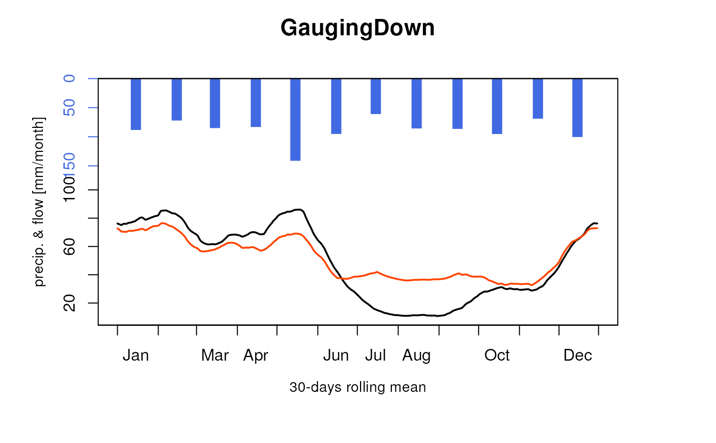
# Compare regimes of the simulation with reservoir and observation of natural flow
plot(OutputsModels,
data.frame(GaugingDown = BasinObs$Qmm[Ind_Run]),
which = "Regime")
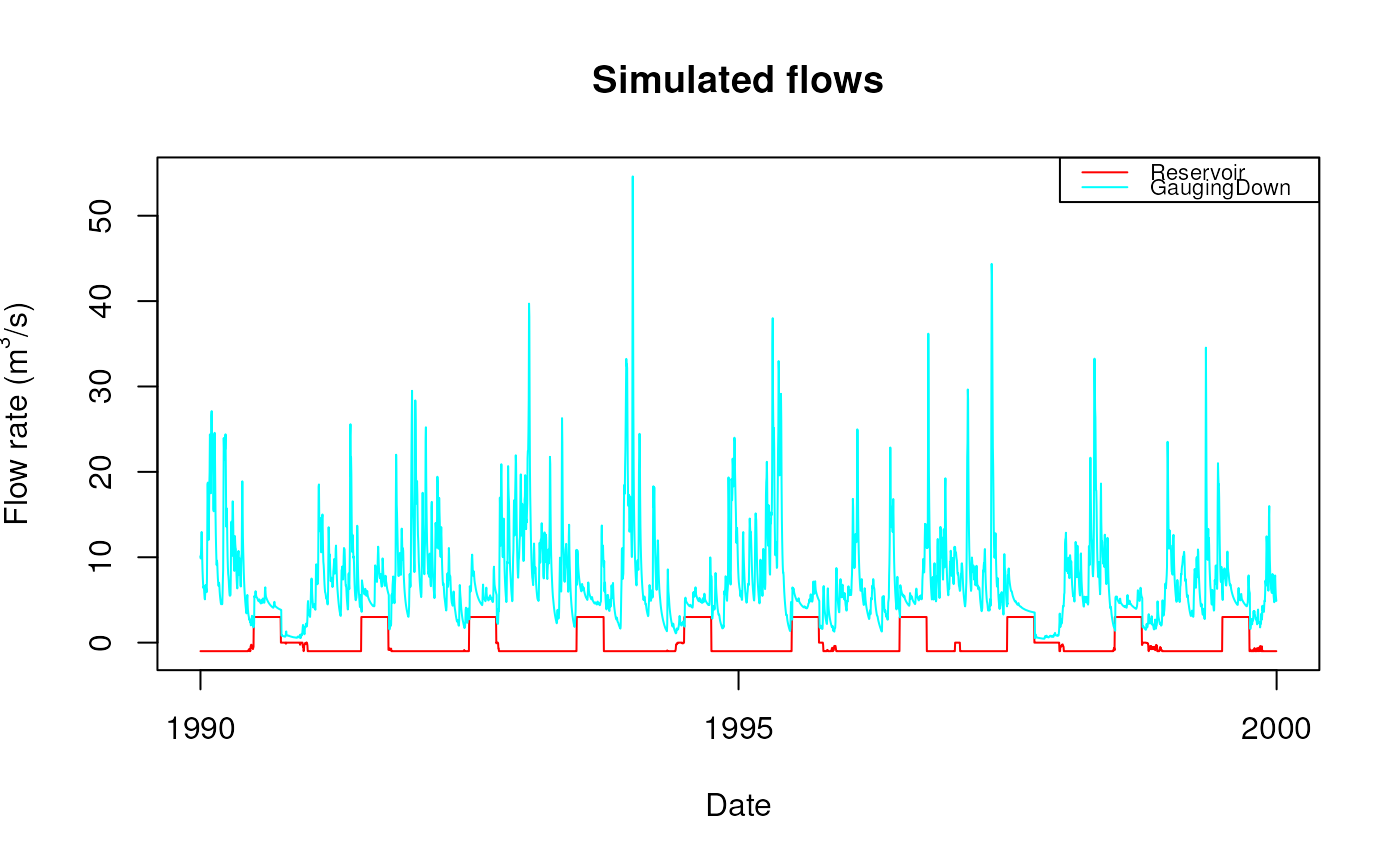
 # Plot together simulated flows (m3/s) of the reservoir and the gauging station
plot(attr(OutputsModels, "Qm3s"))
# Plot together simulated flows (m3/s) of the reservoir and the gauging station
plot(attr(OutputsModels, "Qm3s"))
 ########################################################
# Run the Severn example provided with this package #
# A natural catchment composed with 6 gauging stations #
########################################################
data(Severn)
nodes <- Severn$BasinsInfo
nodes$model <- "RunModel_GR4J"
# Mismatch column names are renamed to stick with GRiwrm requirements
rename_columns <- list(id = "gauge_id",
down = "downstream_id",
length = "distance_downstream")
g_severn <- CreateGRiwrm(nodes, rename_columns)
# Network diagram with upstream basin nodes in blue, intermediate sub-basin in green
plot(g_severn)
# Format CAMEL-GB meteorological dataset for airGRiwrm inputs
BasinsObs <- Severn$BasinsObs
DatesR <- BasinsObs[[1]]$DatesR
PrecipTot <- cbind(sapply(BasinsObs, function(x) {x$precipitation}))
PotEvapTot <- cbind(sapply(BasinsObs, function(x) {x$peti}))
# Precipitation and Potential Evaporation are related to the whole catchment
# at each gauging station. We need to compute them for intermediate catchments
# for use in a semi-distributed model
Precip <- ConvertMeteoSD(g_severn, PrecipTot)
PotEvap <- ConvertMeteoSD(g_severn, PotEvapTot)
# CreateInputsModel object
IM_severn <- CreateInputsModel(g_severn, DatesR, Precip, PotEvap)
#> CreateInputsModel.GRiwrm: Processing sub-basin 54095...
#> CreateInputsModel.GRiwrm: Processing sub-basin 54002...
#> CreateInputsModel.GRiwrm: Processing sub-basin 54029...
#> CreateInputsModel.GRiwrm: Processing sub-basin 54001...
#> CreateInputsModel.GRiwrm: Processing sub-basin 54032...
#> CreateInputsModel.GRiwrm: Processing sub-basin 54057...
# GRiwrmRunOptions object
# Run period is set aside the one-year warm-up period
IndPeriod_Run <- seq(
which(IM_severn[[1]]$DatesR == (IM_severn[[1]]$DatesR[1] + 365*24*60*60)),
length(IM_severn[[1]]$DatesR) # Until the end of the time series
)
IndPeriod_WarmUp <- seq(1, IndPeriod_Run[1] - 1)
RO_severn <- CreateRunOptions(
IM_severn,
IndPeriod_WarmUp = IndPeriod_WarmUp,
IndPeriod_Run = IndPeriod_Run
)
# Load parameters of the model from Calibration in vignette V02
P_severn <- readRDS(system.file("vignettes", "ParamV02.RDS", package = "airGRiwrm"))
# Run the simulation
OM_severn <- RunModel(IM_severn,
RunOptions = RO_severn,
Param = P_severn)
#> RunModel.GRiwrmInputsModel: Processing sub-basin 54095...
#> RunModel.GRiwrmInputsModel: Processing sub-basin 54002...
#> RunModel.GRiwrmInputsModel: Processing sub-basin 54029...
#> RunModel.GRiwrmInputsModel: Processing sub-basin 54001...
#> RunModel.GRiwrmInputsModel: Processing sub-basin 54032...
#> RunModel.GRiwrmInputsModel: Processing sub-basin 54057...
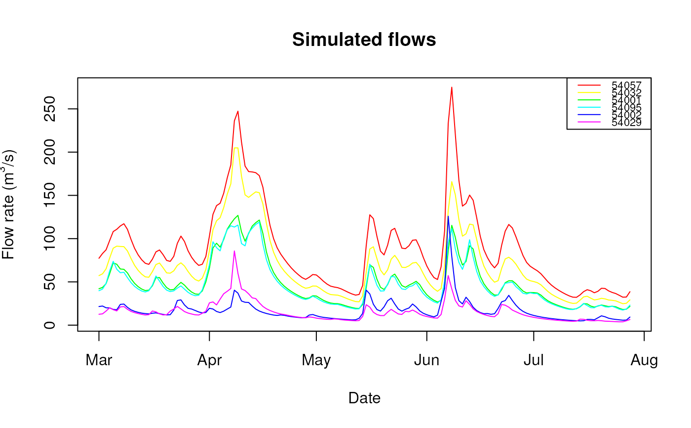
# Plot results of simulated flows in m3/s
Qm3s <- attr(OM_severn, "Qm3s")
plot(Qm3s[1:150, ])
########################################################
# Run the Severn example provided with this package #
# A natural catchment composed with 6 gauging stations #
########################################################
data(Severn)
nodes <- Severn$BasinsInfo
nodes$model <- "RunModel_GR4J"
# Mismatch column names are renamed to stick with GRiwrm requirements
rename_columns <- list(id = "gauge_id",
down = "downstream_id",
length = "distance_downstream")
g_severn <- CreateGRiwrm(nodes, rename_columns)
# Network diagram with upstream basin nodes in blue, intermediate sub-basin in green
plot(g_severn)
# Format CAMEL-GB meteorological dataset for airGRiwrm inputs
BasinsObs <- Severn$BasinsObs
DatesR <- BasinsObs[[1]]$DatesR
PrecipTot <- cbind(sapply(BasinsObs, function(x) {x$precipitation}))
PotEvapTot <- cbind(sapply(BasinsObs, function(x) {x$peti}))
# Precipitation and Potential Evaporation are related to the whole catchment
# at each gauging station. We need to compute them for intermediate catchments
# for use in a semi-distributed model
Precip <- ConvertMeteoSD(g_severn, PrecipTot)
PotEvap <- ConvertMeteoSD(g_severn, PotEvapTot)
# CreateInputsModel object
IM_severn <- CreateInputsModel(g_severn, DatesR, Precip, PotEvap)
#> CreateInputsModel.GRiwrm: Processing sub-basin 54095...
#> CreateInputsModel.GRiwrm: Processing sub-basin 54002...
#> CreateInputsModel.GRiwrm: Processing sub-basin 54029...
#> CreateInputsModel.GRiwrm: Processing sub-basin 54001...
#> CreateInputsModel.GRiwrm: Processing sub-basin 54032...
#> CreateInputsModel.GRiwrm: Processing sub-basin 54057...
# GRiwrmRunOptions object
# Run period is set aside the one-year warm-up period
IndPeriod_Run <- seq(
which(IM_severn[[1]]$DatesR == (IM_severn[[1]]$DatesR[1] + 365*24*60*60)),
length(IM_severn[[1]]$DatesR) # Until the end of the time series
)
IndPeriod_WarmUp <- seq(1, IndPeriod_Run[1] - 1)
RO_severn <- CreateRunOptions(
IM_severn,
IndPeriod_WarmUp = IndPeriod_WarmUp,
IndPeriod_Run = IndPeriod_Run
)
# Load parameters of the model from Calibration in vignette V02
P_severn <- readRDS(system.file("vignettes", "ParamV02.RDS", package = "airGRiwrm"))
# Run the simulation
OM_severn <- RunModel(IM_severn,
RunOptions = RO_severn,
Param = P_severn)
#> RunModel.GRiwrmInputsModel: Processing sub-basin 54095...
#> RunModel.GRiwrmInputsModel: Processing sub-basin 54002...
#> RunModel.GRiwrmInputsModel: Processing sub-basin 54029...
#> RunModel.GRiwrmInputsModel: Processing sub-basin 54001...
#> RunModel.GRiwrmInputsModel: Processing sub-basin 54032...
#> RunModel.GRiwrmInputsModel: Processing sub-basin 54057...
# Plot results of simulated flows in m3/s
Qm3s <- attr(OM_severn, "Qm3s")
plot(Qm3s[1:150, ])
 ##################################################################
# An example of water withdrawal for irrigation with restriction #
# modeled with a Diversion node on the Severn river #
##################################################################
# A diversion is added at gauging station "54001"
nodes_div <- nodes[, c("gauge_id", "downstream_id", "distance_downstream", "area", "model")]
names(nodes_div) <- c("id", "down", "length", "area", "model")
nodes_div <- rbind(nodes_div,
data.frame(id = "54001", # location of the diversion
down = NA, # the abstracted flow goes outside
length = NA, # down=NA, so length=NA
area = NA, # no area, diverted flow is in m3/day
model = "Diversion"))
g_div <- CreateGRiwrm(nodes_div)
# The node "54001" is surrounded in red to show the diverted node
plot(g_div)
# Computation of the irrigation withdraw objective
irrigMonthlyPlanning <- c(0.0, 0.0, 1.2, 2.4, 3.2, 3.6, 3.6, 2.8, 1.8, 0.0, 0.0, 0.0)
names(irrigMonthlyPlanning) <- month.abb
irrigMonthlyPlanning
#> Jan Feb Mar Apr May Jun Jul Aug Sep Oct Nov Dec
#> 0.0 0.0 1.2 2.4 3.2 3.6 3.6 2.8 1.8 0.0 0.0 0.0
DatesR_month <- as.numeric(format(DatesR, "%m"))
# Withdrawn flow calculated for each day is negative
Qirrig <- matrix(-irrigMonthlyPlanning[DatesR_month] * 86400, ncol = 1)
colnames(Qirrig) <- "54001"
# Minimum flow to remain downstream the diversion is 12 m3/s
Qmin <- matrix(12 * 86400, nrow = length(DatesR), ncol = 1)
colnames(Qmin) = "54001"
# Creation of GRimwrInputsModel object
IM_div <- CreateInputsModel(g_div, DatesR, Precip, PotEvap, Qobs = Qirrig, Qmin = Qmin)
#> CreateInputsModel.GRiwrm: Processing sub-basin 54095...
#> CreateInputsModel.GRiwrm: Processing sub-basin 54002...
#> CreateInputsModel.GRiwrm: Processing sub-basin 54029...
#> CreateInputsModel.GRiwrm: Processing sub-basin 54001...
#> CreateInputsModel.GRiwrm: Processing sub-basin 54032...
#> CreateInputsModel.GRiwrm: Processing sub-basin 54057...
# RunOptions and parameters are unchanged, we can directly run the simulation
OM_div <- RunModel(IM_div,
RunOptions = RO_severn,
Param = P_severn)
#> RunModel.GRiwrmInputsModel: Processing sub-basin 54095...
#> RunModel.GRiwrmInputsModel: Processing sub-basin 54002...
#> RunModel.GRiwrmInputsModel: Processing sub-basin 54029...
#> RunModel.GRiwrmInputsModel: Processing sub-basin 54001...
#> RunModel.GRiwrmInputsModel: Processing sub-basin 54032...
#> RunModel.GRiwrmInputsModel: Processing sub-basin 54057...
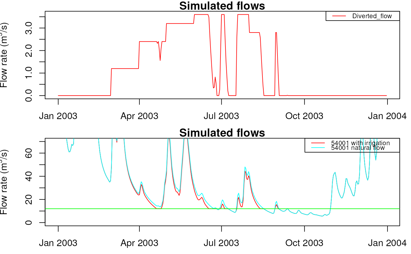
# Retrieve diverted flow at "54001" and convert it from m3/day to m3/s
Qdiv_m3s <- OM_div$`54001`$Qdiv_m3 / 86400
# Plot the diverted flow for the year 2003
Ind_Plot <- which(
OM_div[[1]]$DatesR >= as.POSIXct("2003-01-01", tz = "UTC") &
OM_div[[1]]$DatesR <= as.POSIXct("2003-12-31", tz = "UTC")
)
dfQdiv <- data.frame(DatesR = OM_div[[1]]$DatesR[Ind_Plot],
Diverted_flow = Qdiv_m3s[Ind_Plot])
oldpar <- par(mfrow=c(2,1), mar = c(2.5,4,1,1))
plot.Qm3s(dfQdiv)
# Plot natural and influenced flow at station "54001"
df54001 <- cbind(attr(OM_div, "Qm3s")[Ind_Plot, c("DatesR", "54001")],
attr(OM_severn, "Qm3s")[Ind_Plot, "54001"])
names(df54001) <- c("DatesR", "54001 with irrigation", "54001 natural flow")
plot.Qm3s(df54001, ylim = c(0,70))
abline(h = 12, col = "green")
##################################################################
# An example of water withdrawal for irrigation with restriction #
# modeled with a Diversion node on the Severn river #
##################################################################
# A diversion is added at gauging station "54001"
nodes_div <- nodes[, c("gauge_id", "downstream_id", "distance_downstream", "area", "model")]
names(nodes_div) <- c("id", "down", "length", "area", "model")
nodes_div <- rbind(nodes_div,
data.frame(id = "54001", # location of the diversion
down = NA, # the abstracted flow goes outside
length = NA, # down=NA, so length=NA
area = NA, # no area, diverted flow is in m3/day
model = "Diversion"))
g_div <- CreateGRiwrm(nodes_div)
# The node "54001" is surrounded in red to show the diverted node
plot(g_div)
# Computation of the irrigation withdraw objective
irrigMonthlyPlanning <- c(0.0, 0.0, 1.2, 2.4, 3.2, 3.6, 3.6, 2.8, 1.8, 0.0, 0.0, 0.0)
names(irrigMonthlyPlanning) <- month.abb
irrigMonthlyPlanning
#> Jan Feb Mar Apr May Jun Jul Aug Sep Oct Nov Dec
#> 0.0 0.0 1.2 2.4 3.2 3.6 3.6 2.8 1.8 0.0 0.0 0.0
DatesR_month <- as.numeric(format(DatesR, "%m"))
# Withdrawn flow calculated for each day is negative
Qirrig <- matrix(-irrigMonthlyPlanning[DatesR_month] * 86400, ncol = 1)
colnames(Qirrig) <- "54001"
# Minimum flow to remain downstream the diversion is 12 m3/s
Qmin <- matrix(12 * 86400, nrow = length(DatesR), ncol = 1)
colnames(Qmin) = "54001"
# Creation of GRimwrInputsModel object
IM_div <- CreateInputsModel(g_div, DatesR, Precip, PotEvap, Qobs = Qirrig, Qmin = Qmin)
#> CreateInputsModel.GRiwrm: Processing sub-basin 54095...
#> CreateInputsModel.GRiwrm: Processing sub-basin 54002...
#> CreateInputsModel.GRiwrm: Processing sub-basin 54029...
#> CreateInputsModel.GRiwrm: Processing sub-basin 54001...
#> CreateInputsModel.GRiwrm: Processing sub-basin 54032...
#> CreateInputsModel.GRiwrm: Processing sub-basin 54057...
# RunOptions and parameters are unchanged, we can directly run the simulation
OM_div <- RunModel(IM_div,
RunOptions = RO_severn,
Param = P_severn)
#> RunModel.GRiwrmInputsModel: Processing sub-basin 54095...
#> RunModel.GRiwrmInputsModel: Processing sub-basin 54002...
#> RunModel.GRiwrmInputsModel: Processing sub-basin 54029...
#> RunModel.GRiwrmInputsModel: Processing sub-basin 54001...
#> RunModel.GRiwrmInputsModel: Processing sub-basin 54032...
#> RunModel.GRiwrmInputsModel: Processing sub-basin 54057...
# Retrieve diverted flow at "54001" and convert it from m3/day to m3/s
Qdiv_m3s <- OM_div$`54001`$Qdiv_m3 / 86400
# Plot the diverted flow for the year 2003
Ind_Plot <- which(
OM_div[[1]]$DatesR >= as.POSIXct("2003-01-01", tz = "UTC") &
OM_div[[1]]$DatesR <= as.POSIXct("2003-12-31", tz = "UTC")
)
dfQdiv <- data.frame(DatesR = OM_div[[1]]$DatesR[Ind_Plot],
Diverted_flow = Qdiv_m3s[Ind_Plot])
oldpar <- par(mfrow=c(2,1), mar = c(2.5,4,1,1))
plot.Qm3s(dfQdiv)
# Plot natural and influenced flow at station "54001"
df54001 <- cbind(attr(OM_div, "Qm3s")[Ind_Plot, c("DatesR", "54001")],
attr(OM_severn, "Qm3s")[Ind_Plot, "54001"])
names(df54001) <- c("DatesR", "54001 with irrigation", "54001 natural flow")
plot.Qm3s(df54001, ylim = c(0,70))
abline(h = 12, col = "green")
 par(oldpar)